profiler分析TensorFlow程序性能
1.TensorFlow profiler 功能
从r1.3版本开始, tensorflow 提供profiler模块,参见github上的官网文档
profiler打开tf执行的黑盒,以graph node(神经网络模型简称为graph,其中的节点称为node.)为细粒度,从多个维度、多个层面去统计神经网络运行的时间
和内存消耗,为进一步优化神经网络模型的运行效率提供最直接的数据依据。功能如下:
- 分析 TensorFlow 模型架构。
- 参数量、tensor的shape、浮点运算数、运算设备等。
- 分析 multiple-steps 模型性能。
- 执行时间,内存消耗。
- 自动 分析及建议。
- 训练加速设备使用情况的检查
- 较耗时op的检查
- op配置的检查
- 分布式runtime检查(非OSS)
2.profiler 主要步骤
profiler分为数据搜集和数据显示两个主要步骤。
数据收集
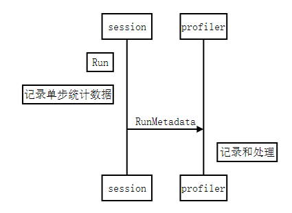
- graph node的每一次执行,记录单步统计数据,主要是执行时间和占用内存,格式参见step_stats.proto,作为原始的最小粒度统计数据源;
- 每一次session.Run(),所有执行到的graph node的统计数据,都集中汇总保存到 RunMetadata 数据结构中;
- 用户程序把每一次搜集到的 RunMetadata 添加到profiler实例,做数据累计和加工处理。
数据显示: 数据的过滤、视图组织和显示输出
部分规则需要用户自己指定:
- 数据的过滤: 比如graph node过滤条件、 显示的字段、排序方式等。
- 四种视图: 对应显示节点之前的不同组织方式。
- scope:应该是 python 层代码中用
tf.name_scope()包起来的视图 - graph:TensorFlow 计算图的视图
- op:把 TensorFlow 计算图再细化一层
- code:Python 代码视图
- scope:应该是 python 层代码中用
- 视图输出方式:
- time line : 输出JSON events file, 再用chrome浏览器tracing功能进行查看,可视性很棒。
- stdout : 标准输出设备打印。
- pprof file: 输出pprof的文件格式,再用pprof工具查看。
- file: 输出到普通的文本文件。
视图和输出方式,可以自由组合,除了部分特例不能输出,比如op view 不支持time line输出,只有code view能够输出pprof格式的文件等,
详细规则参见 Options
2.快速教程
首先,确认下载安装了 r1.3 以上的tensorflow。网络模型使用mnist.py .
import相关的包
1 | import tensorflow as tf |
定义网络模型,创建session.、
网络模型为 hidden1 + hidden2 + softmax 三层架构, hidden1和hidden2都是(Wx+b)->Relu的路径。 默认都运行在gpu:0 上。
1 | # placeholder |
创建tfprofiler实例,作为记录、处理和显示数据的主体
1 | profiler = model_analyzer.Profiler(graph=sess.graph) |
定义trace level为FULL_TRACE,这样我们才能搜集到包括GPU硬件在内的最全统计数据
1 | run_options = tf.RunOptions(trace_level = tf.RunOptions.FULL_TRACE) |
创建RunMetadata, 用于在每次session.Run()时汇总统计数据
1 | run_metadata = tf.RunMetadata() |
循环执行session.Run(),搜集统计数据并添加到tfprofiler实例中
1 | mnist = input_data.read_data_sets(train_dir='./',fake_data=False) |
接下来我们就可以显示统计视图了
定义显示option 和 视图方式
定义显示option 和 视图方式
option用于设置过滤条件、显示字段,完整option 参见Options,常用设置项目:
- account_type_regexes:采用Google RE2规则的正则表达式,
过滤要显示的node的op type 和 device,比如 ‘.MatMul.‘, ‘.Conv2D’, ‘.gpu:0’等。 - select:要显示的字段:
[bytes|micros|accelerator_micros|cpu_micros|params|float_ops|occurrence|tensor_value|device|op_types|input_shapes] - order_by: 显示结果排序方式:
[name|depth|bytes|micros|accelerator_micros|cpu_micros|params|float_ops|occurrence] - output: 输出方式:stdout, file 或者 timeline。
- step: 显示在某个具体的Run() step的统计值. 缺省值-1,显示所有步骤的平均值。
一般来说, option和试图总是结合起来使用,这里举几个典型应用例子:
例子1:grpah view显示每个graph node运行时间,并输出到timeline
1 | #统计内容为每个graph node的运行时间和占用内存 |
我们得到第70步的详细time line结果,打开chrome浏览器,输入about:tracing, 然后load “/tmp/mnist_profiler.json” 文件,这时候可以看见time line的显示结果。

- 横向是时间轴:各device对graph node的kernel调度时间轴、执行时间轴。
- 整个graph中所有执行到的node在devices上的运行分布。由于本例中node缺省使用gpu:0,所以cpu:0上没有执行node的分布。
- 一个kernel的执行包括调度和执行两个阶段,这两个阶段是异步操作,所以我们看到同一个时间点, 当 gpu:0/stream 上还在执行hidden1/Matmul, 而gpu:0已经开始调度下一个node: hidden1/add 的kernel, 这样实现了最大程度上不同node 间的并发。
- 你可以通过tf.device()将部分node分布到其他gpu上或者cpu上,看看做model parallel的结果。
例子2:scope view显示模型中的参数数量分布
通过这种方式,查看各个layer中参数的总数,以控制模型的大小和参数分布。
1 | #统计内容为所有trainable Variable Op |
我们得到param数量从高到低的排序显示:
1 | ==================Model Analysis Report====================== |